End to end machine learning project to predict house prices

Source code

In this project, I am going to predict the price of a house using its 9 features. Basically i am solving the Kaggle Competition. To complete this ML project we are using the supervised machine learning regression algorithm. Then i will deploy the model using Flask in order to be available for the end-users so they can make use of it.

Introduction

Predictive models for determining the sale price of houses in cities like Bengaluru is still remaining as more challenging and tricky task. The sale price of properties in cities like Bengaluru depends on a number of interdependent factors. Key factors that might affect the price include area of the property, location of the property and its amenities. In this project, I first build a model using sklearn and linear regression using banglore home prices dataset from Kaggle. Second step is to save the trained model and deployed on Flask server, so this server can use the model to respind http requests. Third component is to build an web page in html, css and javascript that allows user to enter home square ft area, bedrooms etc and it will call python flask server to retrieve the predicted price. During this project I covers almost all data science concepts such as data loading and cleaning, outlier detection and removal, feature engineering, dimensionality reduction, gridsearchcv for hyperparameter tunning, k fold cross validation etc.

Inspiration

Exploratory Data Analysis

The train and test data will consist of various features that describe that property in Bengaluru. Each row contains fixed size object of features. There are 9 features and each feature can be accessed by its name.

Features:

• Area_type – describes the area
• Availability – when it can be possessed or when it is ready(categorical and time-series)
• Location – where it is located in Bengaluru (Area name)
• Size – in BHK or Bedroom (1-10 or more)
• Society – to which society it belongs
• Total_sqft – size of the property in sq.ft
• Bath – No. of bathrooms
• Balcony – No. of the balcony
• Target variable:
• Price – Value of the property in lakhs(INR)
  

The Dataset is composed with 13320 records. Since there are only 90 Null values, I first cleaned data by dropping all null values. I added new features : Price per square feet Bhk : Bedrooms Hall Kitchen

Dimensionality Reduction

After examination of location feature which is a categorical variable. We noticed that there are 1287 locations. For that I applied dimensionality reduction technique to reduce the number of locations. Any location having less than 10 data points should be tagged as “other” location. In this way, the number of categories can be reduced by a huge amount.

df.location = df.location.apply(lambda x: 'other' if x in location_stats_less_than_10 else x)
len(df5.location.unique())

We passed from 1287 location to only 241 locations. Later on when we do one hot encoding, it will help us with having fewer dummy columns.

Outlier Removal using Business Logic

I started by assuming that normally square ft per bedroom is 300 (i.e. 2 bhk apartment is minimum 600 sqft. If you have for example 400 sqft apartment with 2 bhk than that seems suspicious and can be removed as an outlier. I retain that hypothesis until the facts make it unlikely and then I will remove such outliers by keeping our minimum threshold per bhk to be 300 sqft.

df[df.total_sqft/df.bhk<300]

It is also unusual to have 2 more bathrooms than the number of bedrooms in a home. If you have a 4 bedroom home and even if you have a bathroom in all 4 rooms plus one guest bathroom, you will have a total bath = total bed + 1 max. Anything above that is an outlier or a data error and can be removed.

df[df.bath<df.bhk+2]

Outlier Removal Using Standard Deviation and Mean

df.price_per_sqft.describe()

count 12456.000000
mean 6308.502826
std 4168.127339
min 267.829813
25% 4210.526316
50% 5294.117647
75% 6916.666667
max 176470.588235
Name: price_per_sqft, dtype: float64
Here we find that min price per sqft is 267 rs/sqft whereas max is 12000000, this shows a wide variation in property prices. We should remove outliers per location using mean and one standard deviation. for that i developped a function : remove_pps_outliers then applied to the dataframe.

def remove_pps_outliers(df):
    df_out = pd.DataFrame()
    for key, subdf in df.groupby('location'):
        m = np.mean(subdf.price_per_sqft)
        st = np.std(subdf.price_per_sqft)
        reduced_df = subdf[(subdf.price_per_sqft>(m-st)) & (subdf.price_per_sqft<=(m+st))]
        df_out = pd.concat([df_out,reduced_df],ignore_index=True)
    return df_out

Before going forward, I first visualise for a given location how the 2 BHK and 3 BHK property prices look like.

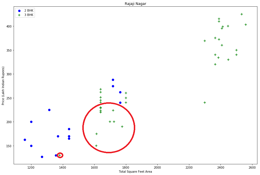
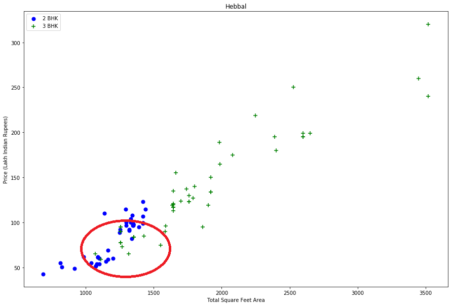Fig. 1: price_per_sqft for 2 BHK and 3 BHK properties for both location “Rajaji Nagar” and “Hebbal” to visualize outliers

From the two plots above, we notice that from the same location, there are some houses with 2 BHK and more expensive than those with 3 BHK. For that reason I should remove properties where for the same location, the price of (for example) 3 bedroom apartment is less than 2 bedroom apartment (with same square ft area). What I will do is for a given location, I will build a dictionary of stats per BHK, i.e. { ‘1’ : { ‘mean’: 4000, ‘std: 2000, ‘count’: 34 }, ‘2’ : { ‘mean’: 4300, ‘std: 2300, ‘count’: 22 }, }

Now we can remove those 2 BHK apartments whose price_per_sqft is less than mean price_per_sqft of 1 BHK apartment. The function I developed to do that process for all the data and all the numbers of BHK that may exists is as following :

def remove_bhk_outliers(df):
    exclude_indices = np.array([])
    for location, location_df in df.groupby('location'):
        bhk_stats = {}
        for bhk, bhk_df in location_df.groupby('bhk'):
            bhk_stats[bhk] = {
                'mean': np.mean(bhk_df.price_per_sqft),
                'std': np.std(bhk_df.price_per_sqft),
                'count': bhk_df.shape[0]
            }
        for bhk, bhk_df in location_df.groupby('bhk'):
            stats = bhk_stats.get(bhk-1)
            if stats and stats['count']>5:
                exclude_indices = np.append(exclude_indices, bhk_df[bhk_df.price_per_sqft<(stats['mean'])].index.values)
    return df.drop(exclude_indices,axis='index')

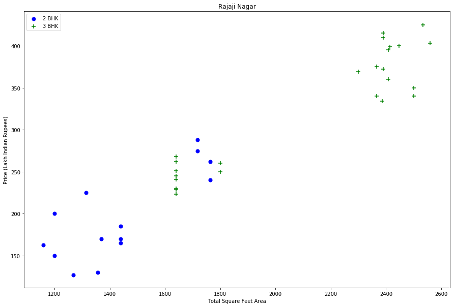
Let’s plot the same scatter chart again to visualize price_per_sqft for 2 BHK and 3 BHK properti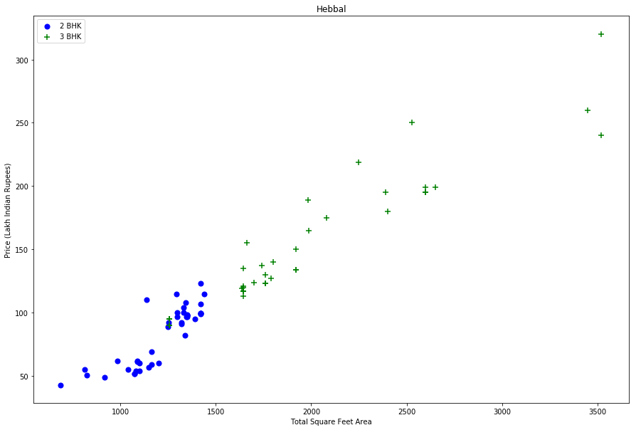es. Fig. 2: price_per_sqft for 2 BHK and 3 BHK properties for both location “Rajaji Nagar” and “Hebbal” after removing outliers The last step in data preprocessing, is to apply One-Hot Encoding to the location feature in order to get a binary representation for the categorical variables.

Machine learning Algorithm and Evaluation

A typical machine learning process involves training different models on the dataset and selecting the one with best performance. However, evaluating the performance of algorithm is not always a straight forward task. There are several factors that can help us determine which algorithm performance best. One such factor is the performance on cross validation set and another other factor is the choice of parameters for an algorithm. Here is my the first attempt to construct a predictive model for evaluating the price based on factors that affects the price. I first split the dataset into train and test dataset.

from sklearn.model_selection import train_test_split
X_train, X_test, y_train, y_test = train_test_split(X,y,test_size=0.2,random_state=10)

Then I fit the linear regression model to the train dataset, next I evalutated the model and got a score of 0.86

from sklearn.linear_model import LinearRegression
lr_clf = LinearRegression()
lr_clf.fit(X_train,y_train)
lr_clf.score(X_test,y_test)

I use K Fold cross validation to measure accuracy of our LinearRegression model

from sklearn.model_selection import cross_val_score
cv = ShuffleSplit(n_splits=5, test_size=0.2, random_state=0)
cross_val_score(LinearRegression(), X, y, cv=cv)

Output : array([0.82702546, 0.86027005, 0.85322178, 0.8436466 , 0.85481502])
Within five iterations we get a score above 80% all the time. This is pretty good but we want to test few other algorithms for regression to see if we can get even better score.

Find best model using GridSearchCV

It is not easy to compare performance of different algorithms by randomly setting the hyper parameters because one algorithm may perform better than the other with different set of parameters. And if the parameters are changed, the algorithm may perform worse than the other algorithms. Therefore, instead of randomly selecting the values of the parameters, a better approach would be to develop an algorithm which automatically finds the best parameters for a particular model. Grid Search is one such algorithm :

from sklearn.model_selection import GridSearchCV
from sklearn.linear_model import Lasso
from sklearn.tree import DecisionTreeRegressor

def find_best_model_using_gridsearchcv(X,y):
    algos = {
        'linear_regression' : {
            'model': LinearRegression(),
            'params': {
                'normalize': [True, False]
            }
        },
        'lasso': {
            'model': Lasso(),
            'params': {
                'alpha': [1,2],
                'selection': ['random', 'cyclic']
            }
        },
        'decision_tree': {
            'model': DecisionTreeRegressor(),
            'params': {
                'criterion' : ['mse','friedman_mse'],
                'splitter': ['best','random']
            }
        }
    }
    scores = []
    cv = ShuffleSplit(n_splits=5, test_size=0.2, random_state=0)
    for algo_name, config in algos.items():
        gs =  GridSearchCV(config['model'], config['params'], cv=cv, return_train_score=False)
        gs.fit(X,y)
        scores.append({
            'model': algo_name,
            'best_score': gs.best_score_,
            'best_params': gs.best_params_
        })

    return pd.DataFrame(scores,columns=['model','best_score','best_params'])

find_best_model_using_gridsearchcv(X,y)

Output :

Model	best_score	best_params
linear_regression	0.847796	{‘normalize’: False}
lasso	0.726738	{‘alpha’: 2, ‘selection’: ‘cyclic’}
decision_tree	0.716064	{‘criterion’: ‘friedman_mse’, ‘splitter’: ‘best’}

Based on above results we can say that LinearRegression gives the best score. Hence we will use that. We export the tested model to a pickle file and start developing Flask application.

Technology and tools used for this project covers

• Python
• Numpy and Pandas for data cleaning
• Matplotlib for data visualization
• Sklearn for model building
• Jupyter notebook, visual studio code as IDE
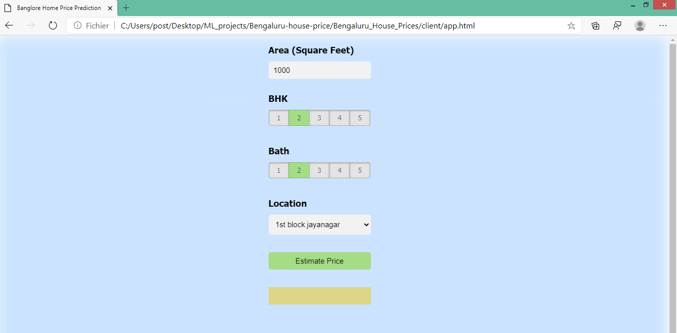
• Python flask for http server
• HTML/CSS/Javascript for UI